Analysis
Operations
Several operations are available within clustertools to perform large scale changes to a StarCluster, primarily related to unit and coordinate system changes. Operations are meant to be called as internal functions (StarCluster.operation_name()), however it is also possible to call operations as external functions (operation_name(StarCluster) if preferred. No information is returned when an operation is called.
A change of units or coordinate system can be implemented using:
>>> cluster.to_galaxy()
>>> cluster.to_kpckms()
It is important to note that the operation analyze is called after a change in either units or coordinate system, such that the properties of the cluster are updated. While resorting won’t occur during a unit change, if resorting is not required when performing a coordinate change use sortstars=False.
>>> cluster.to_galaxy(sortstars=False)
All available operations are listed below.
Functions
|
Convert stellar positions/velocities, centre of mass, and orbital position and velocity to pc and km/s |
|
Convert stellar positions/velocities, centre of mass, and orbital position and velocity to kpc and km/s |
|
Convert stellar positions/velocities, centre of mass, and orbital position and velocity to Nbody units |
|
Convert stellar positions/velocities, centre of mass, and orbital position and velocity to pc and pc/Myr |
|
Convert stellar positions/velocities, centre of mass, and orbital position and velocity to kpc and kpc/Gyr |
|
Convert to on-sky position, proper motion, and radial velocity of cluster |
|
Convert stellar positions/velocities, centre of mass, and orbital position and velocity to galpy units |
|
Convert stellar positions/velocities, centre of mass, and orbital position and velocity to Walter Dehnen Units |
|
Convert stellar positions/velocities, centre of mass, and orbital position and velocity to AMUSE Vector and Scalar Quantities |
|
Convert stellar positions/velocities, centre of mass, and orbital position and velocity fronm AMUSE Vector and Scalar Quantities to pckms |
|
Convert stellar positions/velocities, centre of mass, and orbital position and velocity to user defined units |
|
Convert binary star semi-major axis and periods to solar radii and days |
|
Convert binary star semi-major axis and periods to solar radii and days |
|
Shift coordinates such that origin is the centre of mass |
|
Shift coordinates to clustercentric reference frame |
|
Shift coordinates to galactocentric reference frame |
|
Calculate on-sky position, proper motion, and radial velocity of cluster |
|
Shift cluster to origin as defined by keyword |
|
Save cluster's units and origin |
|
return cluster to a specific combination of units and origin |
|
Assign new conversions for real mass, size, and velocity to Nbody units |
|
Add a degree of rotation to an already generated StarCluster |
|
Adjust stellar velocities so cluster is in virial equilibrium |
Functions
A long list of functions exist within clustertools that can be called to measure a speciic property of the StarCluster. When functions are called internally (StarCluster.function_name()), changes are made to variables within StarCluster and the calculated value is returned. In some cases one may wish to call a function externally (function_name(StarCluster)) to return additional information or to avoid making changes to StarCluster . For example, a cluster’s half-mass relaxation time can be called internally via:
>>> cluster.half_mass_relaxation_time()
where the variable cluster.trh now represents the half-mass relaxation time. Alternatively, the cluster’s half-mass relaxation time can be called externally via:
>>> trh=half_mass_relaxation_time(cluster)
When called externally, cluster.trh is not set.
Some functions, including mass_function and eta_function can be applied to a sub-population of the cluster. They have an array of input parameters that allow for only certain stars to be used. For example, to measure the mass function of stars between 0.1 and 0.8 Msun within the cluster’s half-mass radius one can call:
>> cluster.mass_function(mmin=0.1,mmax=0.8,rmin=0.,rmax=cluster.rm)
Note that, due to the internal call, the slope of the mass function will be returned and set to cluster.alpha. If additional information is required, like the actual mass function bins m_mean, the number of stars in each bin m_hist, the mass function dM/dN dm, and slope of the mass function and its error alpha, ealpha, and finally the y-intercept and error of the linear fit to the mass function in logspace yalpha,``eyalpha`` the function can be called externally:
>>> m_mean, m_hist, dm, alpha, ealpha, yalpha, eyalpha = mass_function(cluster,
        mmin=0.1,mmax=0.8,rmin=0.,rmax=cluster.rm)
Other constraints include velocity (vmin,``vmax``), energy (emin,``emax``) and stellar evolution type (kwmin,``kwmax``). Alternatively a boolean array can be passed to index to ensure only a predefined subset of stars is used.
Finally, cluster properties that depend on the external tidal field, like its tidal radius (also referred to as the Jacobi radius) or limiting radius (also referred to as the King tidal radius), can be calculated when the orbit and external tidal field are given. The defualt external galpy potential is always None. A simple Galactic model to use would be MWPotential2014 model, which is an observationally motived represetnation of the Milky Way that can be imported via:
>>> from galpy.potential import MWPotential2014
>>> pot = MWPotential2014
It is always possible to define a different galpy potential using the pot variable where applicable. See https://docs.galpy.org/en/latest/reference/potential.html for a list of potentials in galpy.
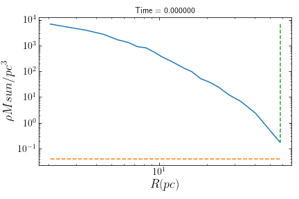
For example, the limiting radius of a cluster (radius where the density falls to background) can be measured via:
>> from galpy.potential import MWPotential2014 >> cluster.rlimiting(pot=MWPotential2014, plot=True)
Since plot=True, a figure showing the cluster’s density profile and the background density in MWPotential at the cluster’s position is returned in order to view exactly where the limiting radius is. cluster.rl is now set equal to the the measured limiting radius. See the full list of functions and their input parameters to see what other functions have the plot option as well.
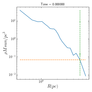
Alternatively, one can define a different galpy potential and make the calculation again:
>> from galpy.potential import LogarithmicHaloPotential >> cluster.rlimiting(pot=LogarithmicHaloPotential,plot=True)
If the cluster’s orbit is not known it is possible to set a galactocentric distance using rgc.
The calculation of a cluster’s tidal radius also requires knowledge of the external tidal field, and can be calculated via:
>> from galpy.potential import MWPotential2014 >> cluster.rtidal(pot=MWPotential2014, plot=True)
It is, however, worth noting that rtidal has two additional arguments that can improve your calculation of the tidal radius. It may be the case that not all of your particles are technically part of the star cluster. In this case, you could consider setting rtiterate and rtconverge. When set, clustertools will first calculate rt using all the particles in the StarCluster. It will then recalculate rt using only the particles within the initial estimate of the tidal radius. This process will occur rtiterate times or until the ratio of the new tidal radius to the previous tidal radius is greater than than rtconverge. For example, rtconverge=0.9 means the tidal radius has changed by less than 10 percent between iterations. Alternatively, if one knew which stars were bound to the cluster you could define a sub_cluster of bound particles and calculate it’s tidal radius or pass a boolean array to rtidal to inform it which stars to use in the calculate of rt.
All functions, with the exception of calculating the cluster’s tidal radius, can be called using projected valeus with projected=True. When called internally, a function call will default to whatever StarCluster.projected is set to if projected is not given.
The complete list of available functions are tabulated below in their external form.
Functions
|
Find the cluster's centre |
|
Find cluster's centre of density |
|
Find the centre of mass of the cluster |
|
Calculate the relaxation time (Spitzer & Hart 1971) within a given radius of the cluster |
|
Calculate the half-mass relaxation time (Spitzer 1987) of the cluster - Spitzer, L. |
|
Calculate the core relaxation time (Stone & Ostriker 2015) of the cluster |
|
Calculate kinetic and potential energy of every star Parameters ---------- cluster : class StarCluster instance specific : bool find specific energies (default: True) ids: bool or int if given, find the energues of a subset of stars defined either by an array of star ids, or a boolean array that can be used to slice the cluster. (default: None) projected : bool use projected values (default: False) softening : float Plummer softening length in cluster.units (default: 0.0) full : bool calculate distance of full array of stars at once with numbra (default: True) parallel : bool calculate distances in parallel (default: False) Returns ------- kin,pot : float kinetic and potential energy of every star if the i_d argument is not used. If i_d argument is used, return an arrays with potential and kinetic energy in the same shape of i_d History ------- 2019 - Written - Webb (UofT) 2022 - Updated with support for multiple ids or an idexing array - Erik Gillis (UofT). |
|
Find distance to closest star for each star - uses numba |
|
Calculate lagrange radii of the cluster by mass |
|
Calculate virial radius of the cluster - Virial radius is calculated using either: -- the average inverse distance between particles, weighted by their masses (default) -- the radius at which the density is equal to the critical density of the Universe at the redshift of the system, multiplied by an overdensity constant Parameters ---------- cluster : class StarCluster method : str method for calculating virial radius (default: 'inverse_distance', alternative: 'critical_density') |
|
Calculate virial radius of the cluster - Virial radius is defined as the inverse of the average inverse distance between particles, weighted by their masses -- Definition taken from AMUSE (www.amusecode.org) -- Portegies Zwart S., McMillan S., 2018, Astrophysical Recipes; The art ofAMUSE, doi:10.1088/978-0-7503-1320-9 |
|
Calculate virial radius of the cluster |
|
Find mass function over a given mass range |
|
Find a tapered mass function over a given mass range |
|
NAME: Find power slope of velocity dispersion versus mass |
|
NAME: Find meq from velocity dispersion versus mass |
|
NAME: Find the kinematic concentration parameter ck |
|
Calculate core radius of the cluster -- The default method (method='casertano') follows Casertano, S., Hut, P. |
|
Calculate tidal radius of the cluster - The calculation uses Galpy (Bovy 2015_, which takes the formalism of Bertin & Varri 2008 to calculate the tidal radius -- Bertin, G. & Varri, A.L. 2008, ApJ, 689, 1005 -- Bovy J., 2015, ApJS, 216, 29 - riterate = 0 corresponds to a single calculation of the tidal radius based on the cluster's mass (np.sum(cluster.m)) -- Additional iterations take the mass within the previous iteration's calculation of the tidal radius and calculates the tidal radius again using the new mass until the change is less than 90% - for cases where the cluster's orbital parameters are not set, it is possible to manually set rgc which is assumed to be in kpc. |
|
Calculate limiting radius of the cluster |
Profiles
A common measurement to make when analysing star clusters is to determine how a certain parameter varies with clustercentric distance. Therefore a list of commonly measured profiles can be measured via clustertools. Unlike operations and functions, profiles can ONLY be called externally. For example, the density profile of a cluster can be measured via:
>>> rprof, pprof, nprof= rho_prof(cluster)
where the radial bins rprof, the density in each radial bin pprof, and the number of stars in each bin nprof will be returned. It is also possible to normalize the radial bins of a profile using normalize=True by the half-mass radius or the projected half-mass radius if projected=True via:
>>> rprof, pprof, nprof= rho_prof(cluster,normalize=True)
Note, when measuring the radial variation in the mass function or the degree of energy equipartition, delta_alpha and delta_eta are calculated with clustercentric radii normalized by the effective radius. Whether or not normalization is True of False only affects whether the returned radial bins are normalized or not.
One feature that is available for all profiles is the ability to plot the profile using plot=True. For example, calling
>>> lrprofn, sigvprof= sigv_prof(cluster,plot=True)
returns the below figure
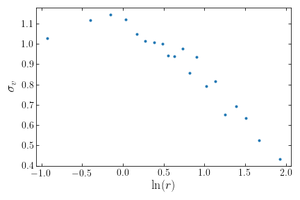
Some editing can be done to the plot via key word arguments (see Utilities for information regarding making figures with clustertools)
All profiles can also just be measured for a select subpopulation of stars based on mass (mmin,``mmax``), radius (rmin,``rmax``), velocity (vmin,``vmax``), energy (emin,``emax``) and stellar evolution type (kwmin,``kwmax``). Alternatively a boolean array can be passed to index to ensure only a predefined subset of stars is used.
All available profiles are listed below.
Functions
|
Measure the density profile of the cluster |
|
Measure the mass profile of the cluster |
|
Measure the radial variation in the mass function |
|
Measure the radial variation in the velocity dispersion |
|
Measure the anisotropy profile of the cluster |
|
Measure the radial variation in the mean velocity |
|
Measure the radial variation in the mean squared velocity |
|
Measure the radial variation in eta |
|
NAME: |
Orbit
In cases where the StarCluster does not evolve in isolation, it is possible to specify both the cluster’s orbit and the the external tidal field. When orbital and tidal field information are provided, clustertools makes use of galpy to help visualize and analyse the cluster’s orbital properties. Hence Bovy (2015) must be cited anytime a clusertools function makes use of the external tidal field and/or the cluster’s orbit.
As discussed in Initialization , the default value for the solar distance (ro) is 8.275 kpc (Gravity Collaboration, Abuter, R., Amorim, A., et al. 2020 ,A&A, 647, A59), the [U,V,W] motion of the Sun is set to [-11.1,12.24,7.25] (Schönrich, R., Binney, J., Dehnen, W., 2010, MNRAS, 403, 1829) and the velocity of the local standard of rest (vo) is 239.23 km/s. The choice of vo is such that vo + V is consistent with current estimates of the proper motion of Sagitarius A* (Reid, M.J. & Brunthaler, A., ApJ, 892, 1).The height of the Sun above the disk zo is 0.0208 kpc (Bennett, M. & Bovy, J. 2019, MNRAS, 483, 1417). However the below functions all allow for these parameters to be uniquely set.
Similar to functions, orbital analyis can be done using internal calls (which set variables inside the StarCluster class) or externally (which returns information). For example, one can easily initialize and a cluster’s galpy orbit, given its galactocentric coordinates are known, using:
>> cluster.initialize_orbit()
The returned galpy orbit is also stored in cluster.orbit.
galpy orbits can be initialized for individual stars as well via cluster.initialize_orbits(). If cluster.origin is centre or cluster, the orbits are initialized with clustercentric coordinates. If cluster.origin='galaxy' then each stars position in the galaxy is used to initialize the orbit.
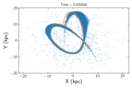
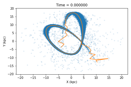
It may also be helpful to have the cluster’s orbital path within +/- dt, especially if looking at escaped stars. Arrays for the cluster’s past and future coordinates can be generated via:
>>> t, x, y, z, vx, vy, vz = orbit_path(cluster,dt=0.1,plot=True)
Since plot=True and dt=0.1, a figure showing all stars in the simulation as well as the orbital path +/- 0.1 Gyr in time is returned.
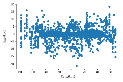
Stars can also be matched to a point along the orbital path, where each stars distance from the path and distance along the path to the progenitor is calculated. This function effectively creates a convenient frame of reference for studying escaped stars.
>>> tstar,dprog,dpath = orbit_path_match(cluster,dt=0.1,plot=True)
Since plot=True, a figure showing dpath vs dprog is returned.
Finally, clusters can be interpolated to past or future points in time. To interpolate a cluster 1 Gyr forward in time use:
>>> cluster.orbit_interpolate(1.0,do_tails=True,rmax=0.1)
By default, all stars are simply shifted so the cluster is centred on its new galactocentric position. If one wishes to identify tail stars that have their own orbits interpolated, set do_tails=True as above and provide a criteria for what defines a tail star. In the above example, any star beyond 0.1 cluster.units is a tail star. Other criteria include velocity, energy, kwtype, or a custom boolean array (similar to defining subsets for profiles as disussed above).
If one wishes to interpolate the orbits of stars within the cluster, then use orbits_interpolate with cluster.origin equal to centre or cluster. In this case the galpy potential of the cluster should be provided. A recomended potential would be a Plummer sphere
>>> from galpy.potential import PlummerPotential
>>> cluster.to_galpy()
>>> pot=PlummerPotential(cluster.mtot,b=cluster.rm/1.305,ro=cluster._ro,vo=cluster._vo)
A complete list of all functions related to a cluster’s orbit can be found below.
Functions
|
Initialize a galpy orbit instance for the cluster |
|
Initialize a galpy orbit for every star in the cluster |
|
Interpolate past or future position of cluster and escaped stars |
|
Interpolate past or future position of stars within the cluster |
|
Interpolate past or future position of cluster and escaped stars |
|
Interpolate past or future position of stars within the cluster |
|
Calculate the cluster's orbital path |
|
Match stars to a position along the orbital path of the cluster |
Tidal Tails
Since stars which escape a cluster lead to the formation of tidal tails, which survive as stellar streams long after the cluster has dissolved. For star cluster simulations that keep track of a cluster’s tidal tails, a few methods are included in clustertools to help in their analysis. Since these methods require knoweldge of the cluster’s orbit, they accept ro, vo, zo, and solarmotion as inputs if the values set for the StarCluster are not relevant. Bovy (2015) should also be cited when using tail functions as well.
The first of which is the
to_tailoperation, which rotates the system such that the cluster’s velocity is pointing along the positive x-axis. Calling the operation externally returns each stars coordinates in the rotated system:
>>> x,y,z,vx,vy,vz=to_tails(cluster)
Alternatively, an internal operation call (cluster.to_tail()) defines the parameters `` cluster.x_tail, cluster.y_tail, cluster.z_tail, cluster.vx_tail, cluster.vy_tail, cluster.vz_tail``.
Secondly, since stars that escape the cluster do so with velocities slightly larger or smaller than the progenitor cluster, tidal tails will not follow the cluster’s orbit path. Therefore clustertools can generate a tail path by first matching stars to the cluster’s orbital path (as above) and then binning stars based on their distance from the progenitor along the path. The mean coordinates of stars in each bin marks the tail path. Similar to a cluster’s orbital path, clustertools can also match stars to the tail path as well.
>>> t, x, y, z, vx, vy, vz = tail_path(cluster,dt=0.1,plot=True)
>>> tstar,dprog,dpath = tail_path_match(cluster,dt=0.1,plot=True)
A complete list of all functions related to a cluster’s orbit can be found below.
Functions
|
Calculate positions and velocities of stars when rotated such that clusters velocity vector |
|
Calculate tail path +/- tfinal Gyr around the cluster |
|
Match stars to a position along the tail path of the cluster |