import clustertools as cts
from clustertools.analysis.functions import meq_func
import numpy as np
import matplotlib.pyplot as plt

A new version of galpy (1.8.1) is available, please upgrade using pip/conda/... to get the latest features and bug fixes!
/Users/webbjere/Codes/clustertools/clustertools/analysis/profiles.py:37: FutureWarning: all profiles are setup such that the returned radial bins and profile values are in linear space and not normalized by the effective radius. Previously select profiles had unique returns.
  warnings.warn('all profiles are setup such that the returned radial bins and profile values are in linear space and not normalized by the effective radius. Previously select profiles had unique returns.',FutureWarning)

Functions

Load a snapshot of a cluster in file 00000.dat, which has position units of pc and velocity units of km/s in clustercentric coordinates. Stellar masses are in solar units and were generated using a Salpeter IMF.

cluster=cts.load_cluster('snapshot',filename='00000.dat',units='pckms',origin='cluster',ofilename='orbit.dat',ounits='kpckms')

Once initialized, any function within clustertools can be called internally via cluster.function_name() or externally via output=function_name(cluster). An internal call sets variables within cluster while an external call will return the calculated values but change nothing within cluster.

In the event that the snapshot is not centered, the centre of the cluster can be found via:

cluster.find_centre()

(-0.14946119556654258,
 -0.22087743738380078,
 -0.038780116570714403,
 0.014544487149392757,
 -0.097072929729564258,
 -0.028231116712277449)

which not only returns the position and velocity of the centre of mass, but also sets cluster.xc, cluster.yc, cluster.zc, cluster.vxc, cluster.vyc, cluster.vzc Alternatively, if you don’t want to set any StarCluster variables just call the function externally:

xc,yc,zc,vxc,vyc,vzc=cts.find_centre(cluster)
print(xc,yc,zc)

-0.149461195567 -0.220877437384 -0.0387801165707

It is important to note that, by default, the centre is calculated to be the centre of density. Similar to NBODY6 and phigrape, once the centre of density is found for the entire cluster population, a centralized subset of stars within an ever decreasing radius are used to find the true centre of density. The parameters rmin and nmax set the minimum radius that can encompass the subset of stars and the maximum number of stars within the subset.

Setting density=False will instead find a central subset of stars to find the cluster’s of centre by removing stars beyond nsigma standard deviations of the previously calculated centre. For systems with a large number of escaped stars, which make finding the cluster’s centre difficult, it may also help to tell the function where to start. For example, it is possible to tell the cluster to start looking for the centre 1 pc away from the origin along the x-axis and remove stars beyond two standard deviations via:

cluster.find_centre(xstart=1.,density=False, nsigma=1)

(0.47255599444213536,
 -0.046784905321136626,
 0.03368417753435262,
 0.0073060547641532469,
 -0.05167863301943116,
 -0.0025985741474006487)

Other functions that can be called include:

print('Half-Mass Relaxation Time: ',cluster.half_mass_relaxation_time())
print('Core Relaxation Time: ',cluster.core_relaxation_time())
print('Lagrange Radii: ',cluster.rlagrange())
print('Virial Radius: ',cluster.virial_radius())

Half-Mass Relaxation Time:  50.5231000207
Core Relaxation Time:  19.6957365444
Lagrange Radii:  [0.73326598977617097, 1.0765583789354674, 1.3646287125197105, 1.7124821982817706, 1.9617869129434311, 2.3496933983866723, 3.1257216188480137, 3.9773141578345004, 5.0211933936198365, 8.3242591110873079]
Virial Radius:  2.51937714706

All functions allow for projected values to be used instead:

print('Half-Mass Relaxation Time: ',cluster.half_mass_relaxation_time(projected=True))
print('Core Relaxation Time: ',cluster.core_relaxation_time(projected=True))
print('Lagrange Radii: ',cluster.rlagrange(projected=True))
print('Virial Radius: ',cluster.virial_radius(projected=True))

Half-Mass Relaxation Time:  33.8815120123
Core Relaxation Time:  20.6789810497
Lagrange Radii:  [0.49097752209716733, 0.7013820946414554, 0.95595297621692432, 1.2127055798991366, 1.5030278513713957, 1.8280543898615964, 2.3000812878962309, 3.068226381254116, 4.1294671402214904, 8.1792344411375115]
Virial Radius:  1.57999162536

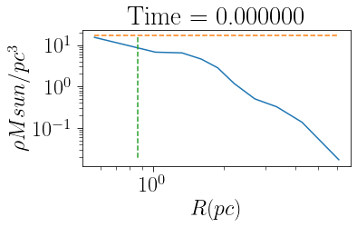
The core radius of the cluster can be calculated by finding where the density drops to 1/3 the central value. The parameter mfrac sets the mass fraction of the cluster that defintes the central region (default 0.1). When projected=True the core radius is where the density drops to 1/2 the central value. rcore also has a plotting feature

cluster.rcore(plot=True)
print(cluster.rc)

0.865233682914

It is also possible to easily measure the mass function and its slope within a given mass range:

m_mean, m_hist, dm, alpha, ealpha, yalpha, eyalpha=cts.mass_function(cluster,mmin=0.1,mmax=0.8,plot=True)

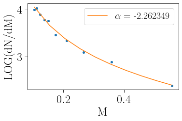
Calling the mass function function internally simply sets the value of alpha and saves the mass range over which alpha was measured with cluster.mmin and cluster.mmax

cluster.mass_function(mmin=0.1,mmax=0.8)

-2.2623485836819826

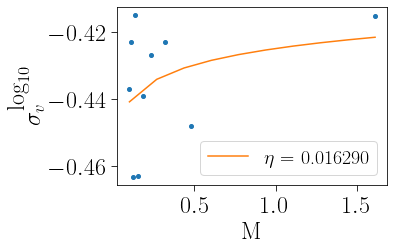
Looking at how velocity dispersion changes as a function of stellar mass is also a proxy for a cluster’s dynamical state, with the power-law slope eta evolving towards (but never reaching) -0.5. An eta of -0.5 corresponds to a state of complete energy equipartition. The external call to eta_function (shown below) and the internal call behave similarly to mass_function above.

m_mean, sigvm, eta, eeta, yeta, eyeta=cts.eta_function(cluster,plot=True)

Alternatively, as per Bianchini et al. 2016, the state of energy equipartition can be probed by the meq parameter

m_mean, sigvm, meq, emeq, ymeq, eymeq=cts.meq_function(cluster,plot=True)

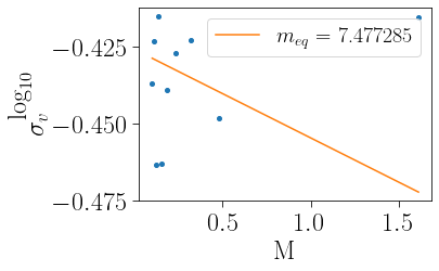
Similarly, as per Bianchini et al. 2018, MNRAS, 475, 96, if you can measure meq you can also measure the kinematic concentration ck, which is the ratio of meq within the half-mass radius to meq at the half mass radius:

cluster.ckin()

1.0000000000004985

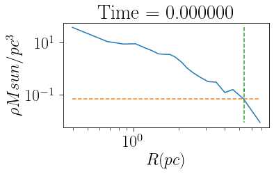
If the cluster’s galactocentric position and velocity are known, then its tidal radius and limiting radius can also be determined. Note when calculating the limiting radius, it is possible to select plot=True to see how the cluster’s density profile reaches the background density.

Note that you need to specify a galpy potential in order to calclated these values. For a Milky Way-like external tidal field, MWPotential2014 from Bovy J., 2015, ApJS, 216, 29 is useful. Different potentials can be used by assigning a galpy potential to the pot variable.

from galpy.potential import MWPotential2014

print('Tidal Radius: ',cluster.rtidal(pot=MWPotential2014))
print('Limiting Radius: ',cluster.rlimiting(pot=MWPotential2014,plot=True))

Tidal Radius:  10.6993452944
Limiting Radius:  5.35685836913

It is also worth noting that it is possible to calculate the tidal radius iteratively. For example, lets assume a snapshot also contains a large number of stars that are likely not members of the cluster. By setting rtiterate>0, clustertools will first calculate the tidal radius using the mass of all stars in the snapshot (rt_old). However it will then calculate the tidal radius using only the mass of stars within the initial calculation (rt_new). This process is repeated rtiterate times or until the ratio of rt_new/rt_old is not less than rtconverge, which by default is 0.9.

print('Tidal Radius: ',cluster.rtidal(pot=MWPotential2014,rtiterate=10))

Tidal Radius:  10.6993452944

Since not all snapshot will contain the energy of each star, clustertools can calculate these values as well by simply calling:

ek, pot=cts.energies(cluster)

If energies were instead called internally, such that cluster.ek,cluster.pot,cluster.etot are set, a subset of stars could be defined that are gravitationally bound (E<0):

cluster.energies()
bound_cluster=cts.sub_cluster(cluster,emax=0.)

Calling energies internally also set the virial parameter Qvir:

print('Qvir = ',cluster.qvir)

Qvir =  -1.40814083302

Finally, in case one needs to know the distance to each stars nearest neighbour:

distance_to_neighbour=cts.closest_star(cluster)
print(np.amin(distance_to_neighbour))

0.032610081984